Use Cases In Detail

This chapter describes the modelling of the adoption of

• alternative drive systems of passenger cars
• PV-battery systems of private house owners
• Power-to-Gas systems

1. Passenger cars

Introduction

The aim of the model is to simulate the annual adoption of alternative drive systems of passenger cars by private persons. With the model results it is possible to compare these results with the targets that originate from energy system scenarios to fulfill the necessary CO2-emission reduction targets.

Empirical data

The modelling approach follows the method of a discrete choice model using data from a representative discrete choice experiment incorporated in an online questionnaire study. The respondents had to choose among three alternative vehicle types (battery-electric (BEV), fuel cell (FCEV) and conventional (diesel/gasoline CV)), which were characterized by following attributes:

• CAPEX
• CO2-tax
• fuel costs
• infrastructure
• range
• well2wheel emissions

Each attribute had two to four attribute levels, which were chosen to represent the bandwidth of the development from today until 2050. The attribute levels rotated within the experiment, so that every participant responded to 10 choice tasks. As the attribute levels differ between different car classes a distinction between three classes was undertaken.

• Class1_small (minis, small cars and compact class)
• Class2_medium (mid-sized cars)
• Class3_upper (upper-sized cars and luxury cars)

Model process

For simulating the adoption

1. The model is initialized
2. The utilities are calculated
3. The probabilities are calculated
4. The change in the car stock is calculated

1. Initialization def __init__() (API)

   • the user chooses between different car classes (Class1_small, Class2_medium, Class3_upper)
   • Data base is initialized (this is not necessary if csv data is read in (self.read_data = True))
   • The starting year is defined according to the car stock data 2018

2. Calculate Utility calculate_utility() (API )

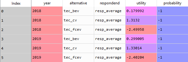
The target of this function is to calculate the total utility of possible alternatives for each respondent. All possible alternatives were created from a set of attribute levels. Via the discrete choice experiment, partial utilities of the respective attribute levels were calculated. The partial utilities were calculated with SAWTOOTH software on the basis of Hierarchical Bayes Estimation (https://www.sawtoothsoftware.com/support/technical-papers/hierarchical-bayes-estimation). The total utilties were calculated as the sum of partial utilities of each attribute level. Partial utilities were provided within the original dataset Data and Database of the discrete choice experiment.

For vehicles, the attributes are specified as a (future attribute development) scenario, in which the car attributes (capex, co2-tax, fuel costs, infrastructure, range and well2well emissions) are specified by means of the predicted? attribute levels for each year from the start_year (2018) until 2050 Class1_small_average__False_S1_moderate_afv_logit_ . By adapting the attribute levels the user can create a new scenario for simulating different technology deployments. As a result, the influence of changing parameters (for example good infrastructure for battery electric vehicles) on the investment decision of alternative vehicle types can be modelled. For a proper functioning of the model ?? it needs to be ensured, that the attribute levels are within the minimum and maximum value of the DCE values. Interpolations of continuous values are possible, extrapolations are not valid. For the discrete attributes (CO2-tax, infrastructure and wel2whell emissions) the partial utilities are directly used from the data set whereas for the continuous attributes (CAPEX, fuel cost, range) the values of the partial utilities are interpolated linearly between two data points.

One option that can be chosen in the car_simulation.py is the inclusion of the NONE option. This operation is only recommended for the calculation of the preference shares but not for the stock model, in which an assumption of the development of the cumulated car stock (as a percentage) can be set as an input parameter. The input data needed as csv or data base query are:

1. alternatives Class1_small_average__False_S1_moderate_afv_logit_
2. query_attribute_level_putility (partial utilities from original dataset)
3. query_utility_none_option (partial utility of none option if enabled)
4. query_attribute_level_per_year (scenario definition from today until 2050 (e.g.attribute_scenanrio =’S1_moderate_afv’))

As a result of the function a pandas.dataframe (utilities_alternatives) is generated. The probability is not calculated in this step (-1 serves as a placeholder). The usage of the average utilities is not recommended, as the results differ distinctly from the usage of the individual utilities. The value resolution and aggregation average is recommended to use for the understanding and further development of the model, as the simulation is much faster than for individual values.

3. Calculate Choice Probability On the basis of the total utilities per alternative per respondent, the preference share for one alternative compared to the other alternatives is calculated. For this purpose, different logics can be applied. One of them needs to be chosen in the car_simulation.py (probability_calc_type = ‘logit’).

First choice calculate_first_choice() (API )

The assumption of this rule is that the respondent chooses the alternative with the highest utility.

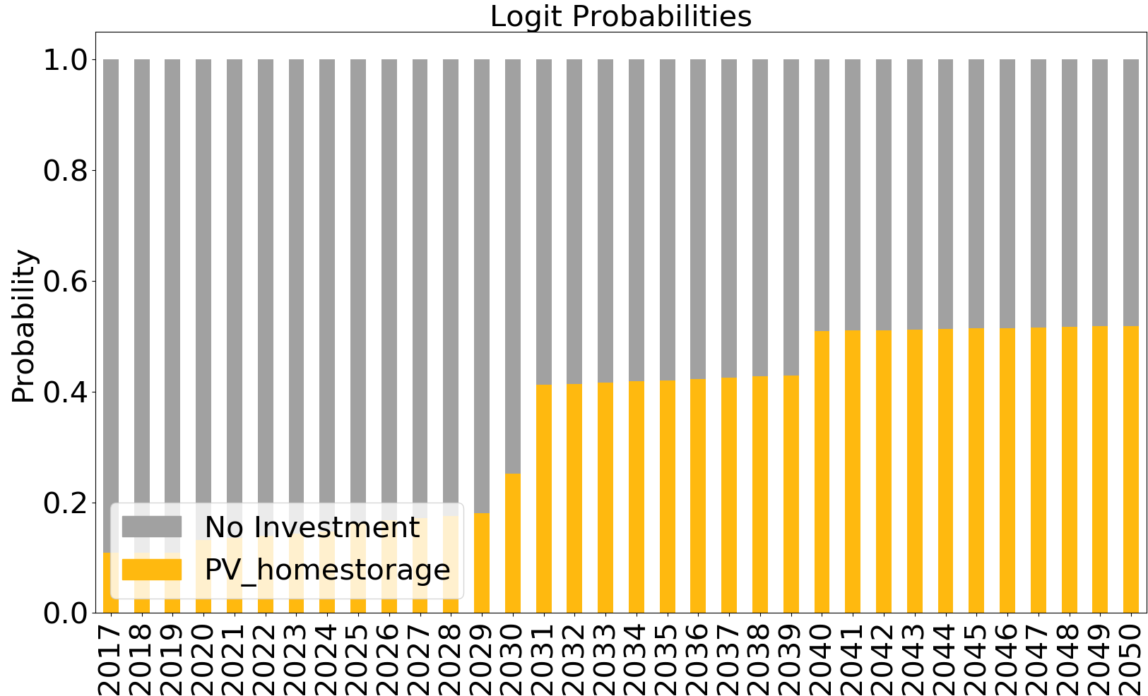
Logit choice probability calculate_logit_probabilities() (API )

Within this rule a share of preference towards each alternative is calculated per respondent. Following the equation:

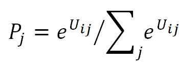
Where i is individual, j is alternative, U is utility and P is the probability

The input data needed as csv or data base query are for both rules:

1. utility_alternatives (result from calculate_utility())
2. main_sub (main_sub = {} (no building of subgroups))

Explanation main_sub: represents a subgroup of the respondents; for example only selecting the respondents that stated to be female for analyzing the influence of person-related factors. Note: The specification only works with database connection. If no connection to the database exists a subgroup of respondents can be manually built in the csv file df_sub.

As a result of one of the decision rules a pandas data frame tb_prob_alternatives is passed and saved (results/tb_prob_alternatives.csv). In addition, a graph with the preference shares is saved (/results/preference_share.png).

4. Stock model stock_model()(API )

Aim of the stock model is the calculation of the total car stock by vehicle type (BEV, FCEV, CV) from 2018 until 2050, on the basis of the preference shares of the individuals. For this purpose, an assumption on the development of the total car stock as a yearly percentage (e.g. growth_scenario = ‘S_constant’) is made to calculate the total number of cars in the next year (stock_sum table), on an annual basis. Additionally, the number of cars that will be deregistered in the actual year is calculated dependent on the age of a car (car_stock table) by vehicle type. To calculate the outage probabilities a Weibull Fit is used on the basis of the historic car stock development (tb_stock) from 2001 to 2018. Having the number of new total car stock for the next year and the outages in the current year, the total number of new cars is calculated. The distribution of the new cars per vehicle type is calculated using the preference shares, that are calculated in either calculate_first_choice() or calculate_logit_probabilities(). The process is repeated sequentially until 2050 on an annual basis. As a result, the csv File stock_sum is saved in the results folder. In addition, the plot stock.png is created and saved.

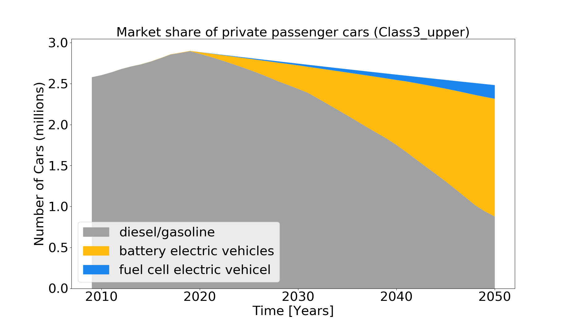
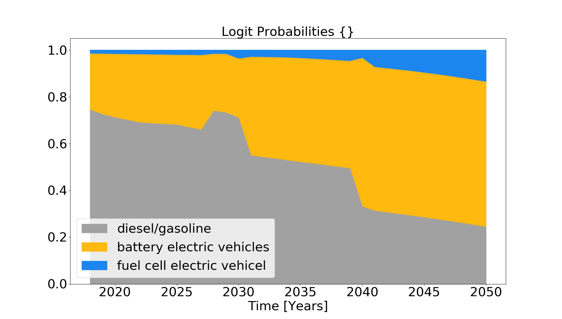
A comparison of the calculated diffusion of alternative driving concepts with shares from cost-minimizing, model-based quantified sector-coupled energy scenarios (e.g. REMod), which include a CO2-emission reduction target is realized on the basis of technology shares. It is plotted and saved in plot share.png and a statement is put in the command prompt :

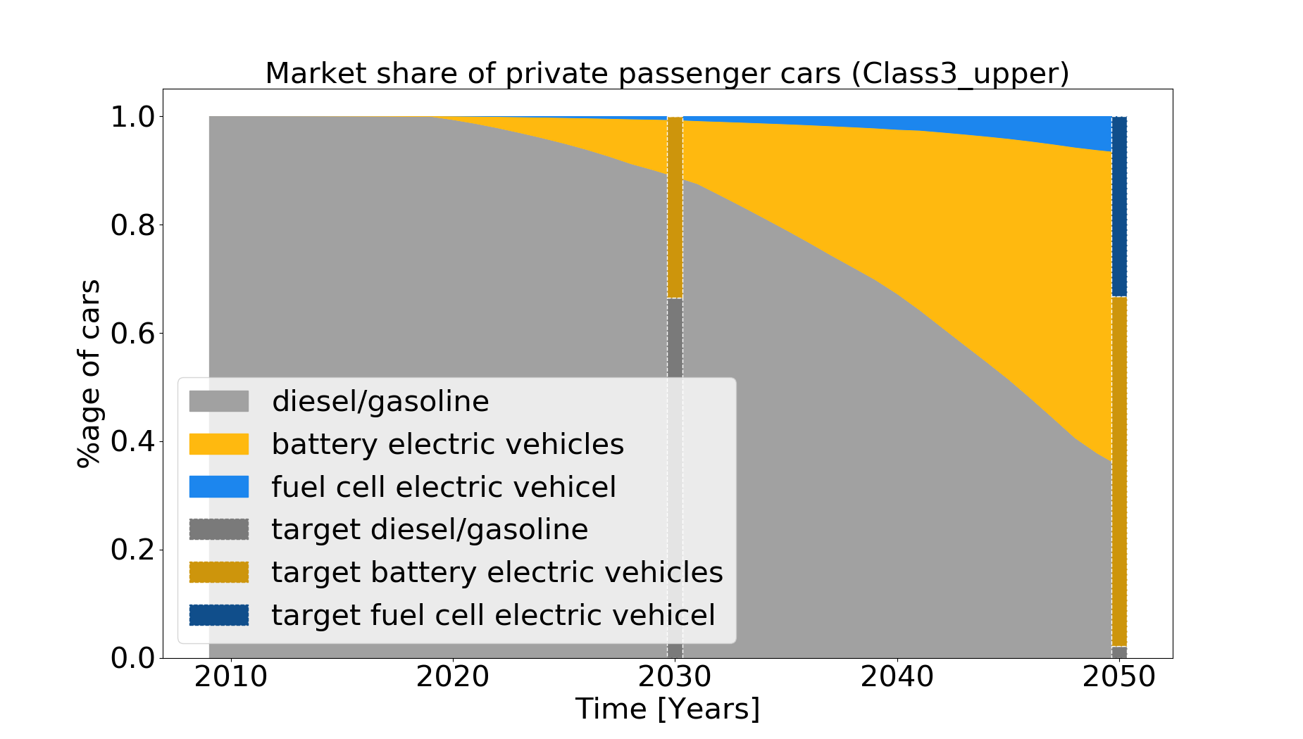
“In 2030, the market share of battery electric vehicles (BV) is 11.46 %. The target of 33.51 % is not achieved. In 2030, the market share of fuel cell electric vehicles (FCEV) is 0.81 %. The target of 0.00 % is achieved. In 2050, the market share of battery electric vehicles (BV) is 57.78 %. The target of 64.52 % is not achieved. In 2050, the market share of fuel cell electric vehicles (FCEV) is 6.76 %. The target of 33.29 % is not achieved.”

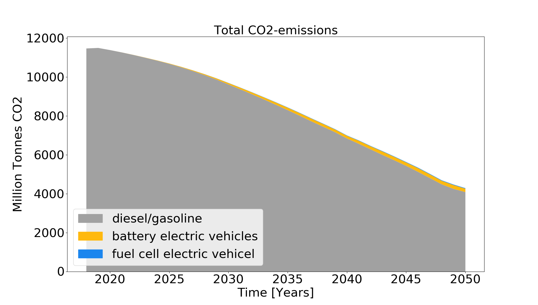
In addition, the CO2-emissions based on assummed passenger kilometers (which is specified in car_simulation.py - e.g average_passenger_kilometers = 20900) are estimated per passenger car and specific emission values. For the calculation of emissions of conventional vehicles, emissions (according to Agora and own assumptions) are calibrated based on the total Pkm in 2018 (source:” Destatis Verkehr in Zahlen”) and 70% (according to Renewbility III) of the total emissions from road transport (UBA) for passenger cars, compared to freight transport. Historic and future specific emissions per construction year and vehicle class are taken as data basis. For calculating emissions of BEV and FCEV assumptions on the specific consumption (kWh/100km) as well as CO2-emissions of the electricity mix [gCO2/kWh]are used to calculate the CO2-emissions.

It has to be mentioned that the specific emissions from literature are much higher than the calibrated values, which shows that uncertainties arise from 1) specific emission values and 2) average driving performance. To adequately calculate the emissions a more detailed model (like TREMOD), which addresses relations between car classes, and driving performance, in terms of road usage, shares of innercity drives, highway drives, overland drives, and further factors would be needed. A plot of theCO2-emissions (CO2_emissions.png) which shows the total estimated CO2-emissions until 2050 is saved. A prompt ”The proportional CO2-emission reduction target of 40-42% in 2030 compared to 1990 in the transport sector is not achieved, as a remaining share of 70% is estimated for 2030 and 40% for 2050” is printed in the console.”

2. PV-homestorage systems

Introduction

The aim of the model is to simulate the purchasing preferences of a PV home storage system (HSS). The alternatives are the purchase of the system or no purchase. The following cases are subdivided, for each of which different attribute levels were determined in the Disctrete Choice Experiment.

Empirical data

• House owner without PV or PV battery system
• House owner with PV system

The modelling approach follows the method of a discrete choice model using data from a representative discrete choice experiment, in which the respondents (house-owners) had to choose among three different types of HSS, which are characterized by following attributes:

• time of realization
• CAPEX
• IRR/Paybacktime
• Degree of autarky
• Environmental impact

Each attribute has three to four attribute levels, which are chosen to represent the bandwidth of the development from today until 2050. The attribute levels are rotating within the experiment, meaning that the experiment was repeated multiple times. The empirical data, containing the individual partial utilities, can be found under the following link:

https://fordatis.fraunhofer.de/handle/fordatis/153

Calculation Steps

To be able to calculate the preferences to buy a HSS system the following calculation steps are undertaken:

The first two steps are performed in the script calc_UCM_economics, steps 3 and 4 in Preferences_HSS.

1. Degree of autarky

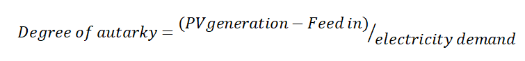
For the calculation without database connection, databaseconnection=False must be set. In this case, Scenario_name = ‘Default_Data’ should be set. The degree of self-sufficiency is one variable for determining the utility of the HSS. Therefore, in a first step, it is determined as a function of various input parameters. The degree of autarky is defined as:

The share of own consumption is defined as:

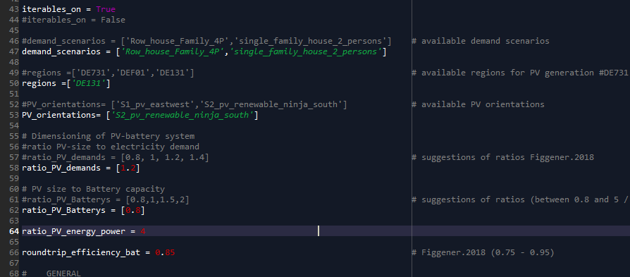
The user input for determining the degree of autarky and own consumption is the ratio of PV system size to demand, the ratio of PV system to battery system (both possible to list for iterative simulation) as well as the ratio of battery capacity to power and the roundtrip efficiency of the battery. The values can be specified as user input in the script.

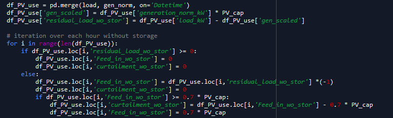
Within the function calculate_PV-battery_use() (API ), the use of the battery is calculated in order to calculate the degree of autarky as well as the own-consumption share for a specific application. The hourly load and the PV generation curve are used as input. The load can be specified for different applications and was determined with the load generator SynPro (https://www.elink.tools/elink-tools/synpro/). The generation time series were determined with renewables.ninja (https://www.renewables.ninja/) and scaled according to the assumed ratio of demand to load. The values are written to the data frame (df_PV_use).

First the operation without storage is calculated. The residual load (residual_load_wo_storage) results from the difference between load and generation (load_kW) - (gen_scaled). From this the grid feed can be calculated without storage (Feed_in_wo_stor). The maximum grid feed-in is limited to 70% of the nominal power according to EEG2014, $9. The curtailment (curtailment_wo_stor) is calculated as the amount of energy that is greater than 70% of the PV output.

The second step is to determine the battery usage. At the first hour the battery is assumed to be empty. The battery is charged if the grid feed is positive (PV surplus) and the state of charge of the previous hour is less than the battery capacity. Limits are the remaining storage level and the charging capacity.

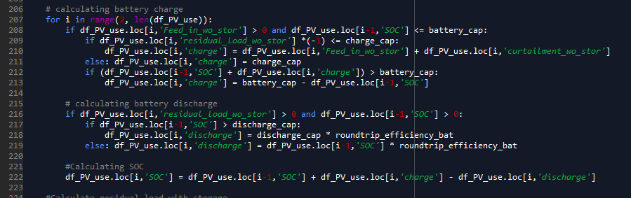
The discharge of the battery always occurs when the residual load is positive (power shortage) and the battery state of charge (SOC) is greater than zero. Thus, the grid feed-in with storage as well as the curtailment can be calculated according to the equations for determining the degree of own consumption and self-sufficiency.

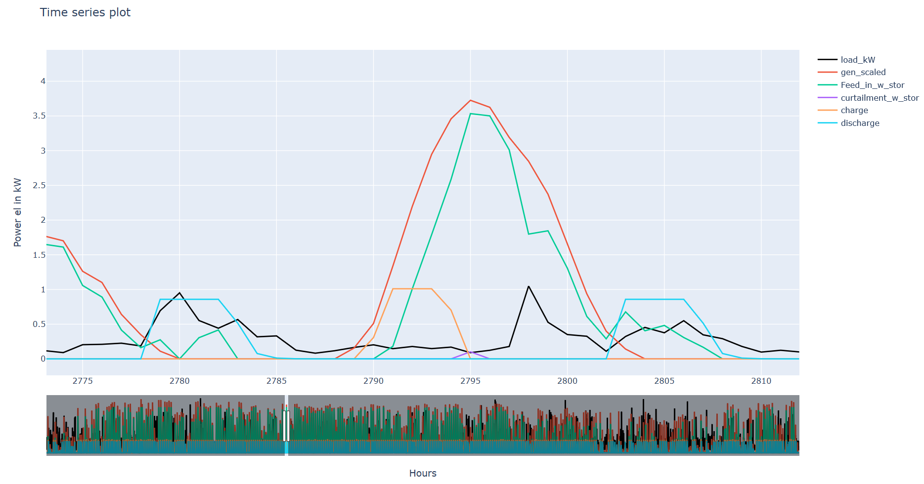
As a result, the hourly storage usage (df_PV_use), the load and generation sums as well as the autarky and own consumption values with and without storage are simulated and saved (result_df). In addition an interactive plot is generated when one system configuration (iterables_on = False) is calculated and opened in the browser.

2. Calculation of economic feasibility (IRR, payback, NPV)

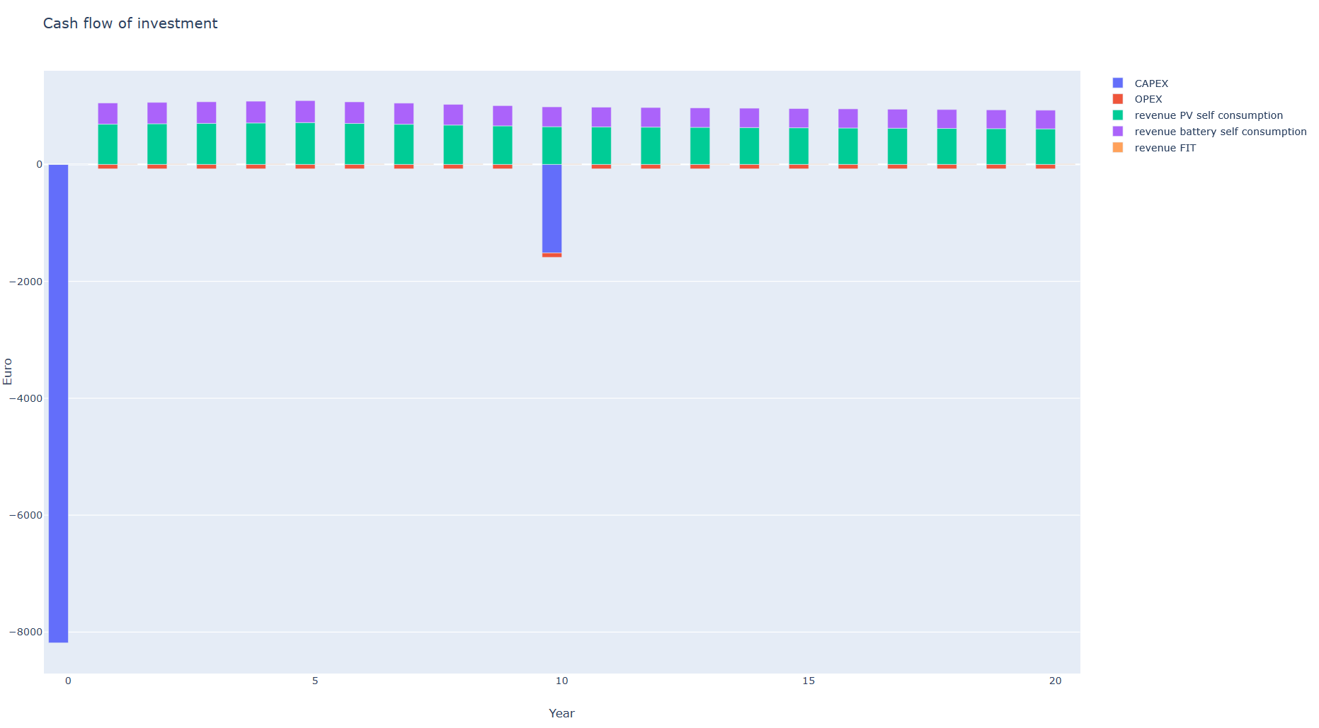
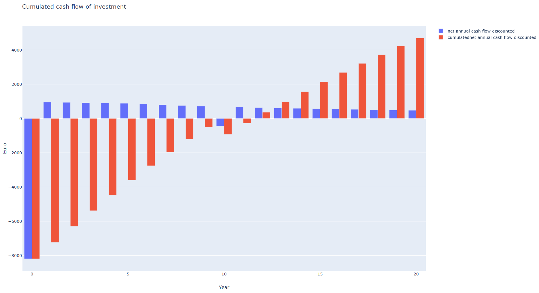
To calculate the economic efficiency of the HSS the cash flow over the technical life of the system is calculated. The cash flow is determined using the calculate_cashflow() (API ) function. When determining the annual PV production, the degradation of the modules is taken into account in the form of an annual factor.

Costs:

Capital costs consist of investment costs (for PV and battery) and installation costs. They are incurred in year 0 and in the year the battery is replaced (defined by technical lifetime of the battery). Further expenses are the annual running costs (OPEX).

Revenues:

The revenues is made up of the PV system’s own consumption, the battery’s own consumption plus VAT (USTG, §19) and the grid feed-in. The annual net cash flow (income - expenditure) is discounted and accumulated using the assumed interest rate. On the basis of the cash flow, various parameters can be determined to calculate the economic efficiency of the system. All relevant data is written to the dataframe df_cashflow. Two plots of the cashflow are generated when only one system configuration and “iterables_on = False” is set and opened in the browser:

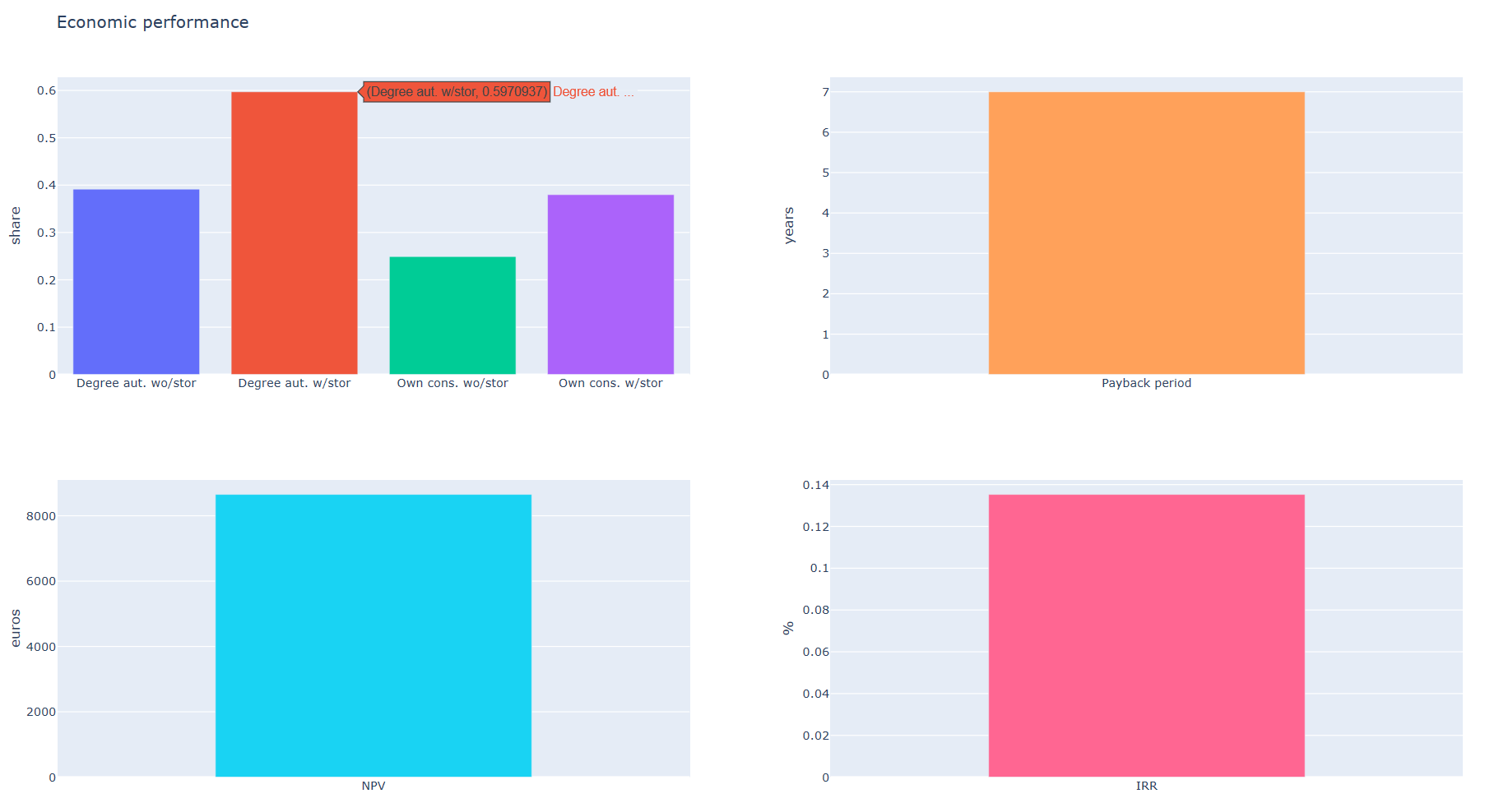
Economic Measures:

The calculate_payback function() determines the payback time.

The function calculate_npv() determines the net present value.

The function calculate_IRR() calculates the internal rate of return.

A plot of the economic measures and the autarky as well as own consumption shares is generated:

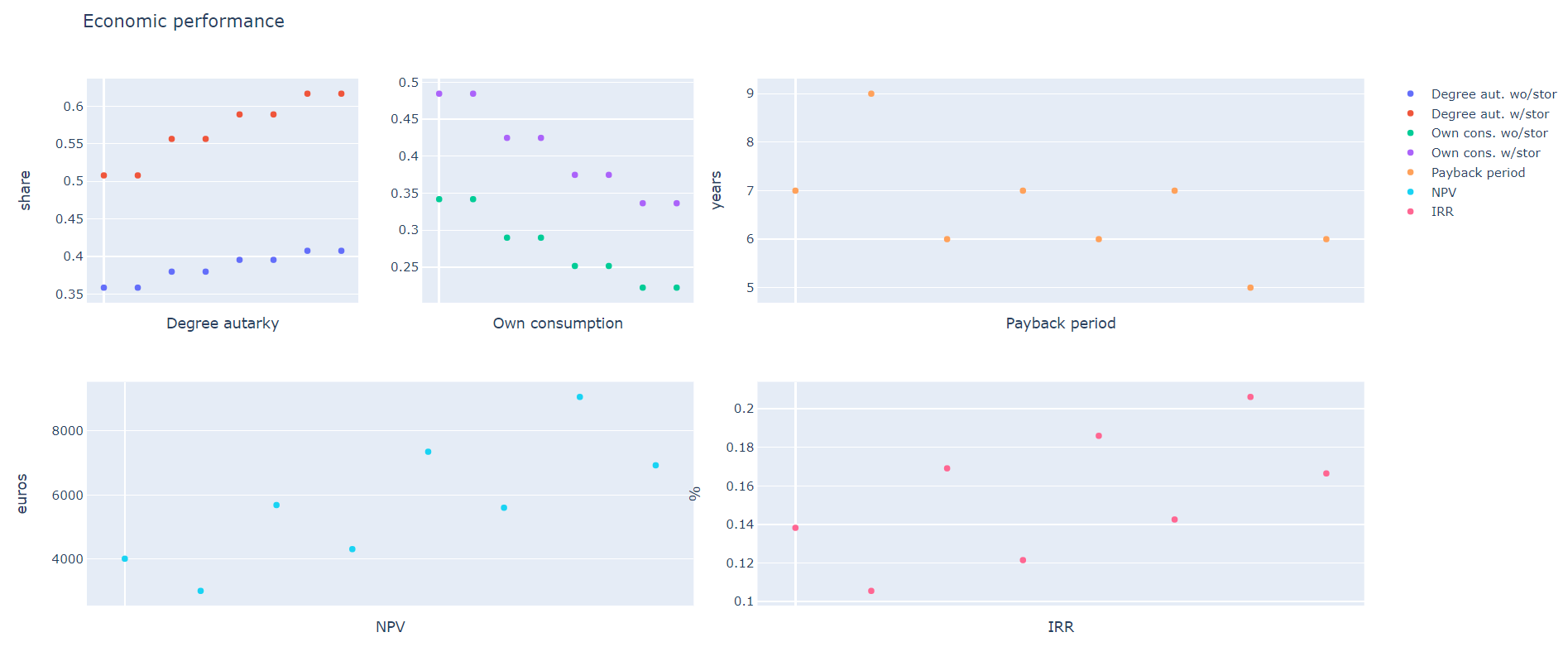
Iterations:

Since there are many possible variations regarding the degree of autarky as well as the economic feasibility of the HSS, the script calc_UCM_economics was designed in a way that a number of parameters can be specified as iteration parameters.

Iterables are:

• start_years (year of calculation e.g. 2020, 2030, etc.)
• demand_scenarios (Defined in database or input file)
• regions (NUTS3-code)
• PV_orientations (East, South-West)
• ratio_PV_demands (e.g. 1)
• ratio_PV_Batterys (e.g. 1)
• WACCs (e.g. 0.018)
• scenario_CAPEX_PVs (Defined in database or input file)
• scenario_CAPEX_bats (Defined in database or input file)
• scenario_FITs (Defined in database or input file)
• scenario_EEXs (Defined in database or input file)
• scenario_consumption_prices (Defined in database or input file)

These can each be specified as a list. Some of the iterables can be entered directly in the script. Others are specified by scenarios stored in the database or in the Input folder. The user can also add his own new scenarios. The results of the iteration are stored in a csv-file (results_df) with the following variables and stored in the model output folder.

result_df = pd.DataFrame(columns = [‘degree_autarky_wo_storage’, ‘degree_autarky_w_storage’, ‘own_consumption_wo_stor’, ‘own_consumption_w_stor’, ‘pay_back’, ‘NPV’, ‘IRR’], index = pd.MultiIndex.from_product(iterables))

For the graphical display of the results (iterables_on = True) should be set.

3&4 Utilities and preference shares

To calculate purchasing preferences, the attribute levels (time of realization, CAPEX, IRR/Paybacktime, Degree of autarky and Environmental impact) are defined in the form of scenarios.The scenarios are based on the possible characteristics of a use case for a particular year. The script calc_UCM_economics was developed for the parameters Degree of Autarky and IRR/Paybacktime in combination with the CAPEX, the results of which can be used for the calculation of preferences. Similar to the case of passenger cars, the numerical values for which interpolation (but no extrapolation) between the values is possible (CAPEX,IRR/Paybacktime,Degree of autarky) and those for which interpolation is not possible (time of realization, environmenatl impact) differ.

The calculation of the utilities is done with the function calculate_utilities(). The calculation of the preference probability can be performed by the functions calculate_logit_probabilities() or calculate_first_choice(). The functions were described in detail for the Use Case passenger cars.

Input Data

For the use case PV-homestorage system there is also the possibility of database connection as well as calculation without database. The setting can be made in the script Preferences_HSS (databaseconnection = True or False).

databaseconnection = False For the calculation without database, the data for the cases (investment_options) homestorage and PV-homestorage are provided, for average and individual resolution. It is explicitly stated that the individual data sets should be used for the calculation. The use of the average data sets leads to a significantly shorter calculation time and can therefore be used for test runs, but they show high inaccuracies. There is also a scenario folder for the two investment options, in which the attributes can be specified by year. Any new scenarios can be added at this point. Note that the attribute level for the continuous attributes must remain within the queried Discrete Choice values and the Discrete takes one of the predefined level values. The name of the csv file must be structured as follows: Scenario_name_attribute_level_per_year.csv

databaseconnection = True

If the database connection is used, for each scenario a new folder is created in the Input folder, which contains all the data that is used.

Results:

As a result, a folder of the scenario is created under Results, which contains a csv file for the partial utilities and preferences. The plot of the preferences is saved.

3. Power-to-Gas

Introduction

In this use case, the diffusion of power to gas in Germany is modelled. For this aim, economic and non-economic determinants for investments are identified and quantified in the form on an indicator which shapes the PtG deployment pathway. This is performed for the sectors ‘mobility’, ‘industry’, ‘injection’ and ‘re-electrification’ seperately. The considered facility sizes are 3.1, 10, 310 and 590 MWel, for the technologies AEL and PEM. For the furture development of energy prices, there are two scenarios, optimistic and pessimistic. At the end this gives a range for the development of PtG. Further different electricity tariffs are considered.

Model process

The diffusion of power to gas is modelled by a logistic function. In the simulation the following steps are undertaken:

1. Calculation of annual diffusion rates from historical data
2. Calculation of determinants
3. Calculation of the modified diffusion

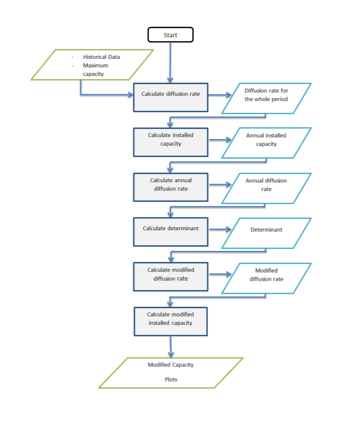
1. Calculation of annual diffusion rate from historical data

In the first step, the logistic function is fitted to the historical data. Therefore the model is explained briefly. Let \(i_{inflect}\) be the year of the inflection point, \(c_{max,s}\) the maximaum capacity in sector \(s\) and \(r_s\) the growth rate of sector \(s\). Then the installed capacity \(c_{i,s}\) of sector \(s\) in year \(i\) is given as the following sum:

\[c_{i,s} = \frac{c_{max,s}}{1 + exp(-(i - i_{inflect}) r_s)}.\]

The maximum capacity and the year of the inflection point can be chosen freely. In the github repository the values are from the REMod study (Sterchele 2019). The rate then is obtained by fitting the above formula to the hhistoric data by the method of least squares. Therefore let \(c_{i,s,hist}\) be the capacity from historical data, then the following term is minimized:

\[\sum_{i = 2008}^{2018} (c_{i,s} - c_{i,s,hist})^2.\]

This yields for each sector an overall growth rate \(r_s\) which gives the logistic function wich fit best the historic data. From this the annual capacities \(c_{i,s}\) can be computet which allows to get the annual growth rate \(r_{i,s,hist}\) by

(1)\[r_{i,s,hist} = \frac{c_{s,i} - c_{s,i-1}}{c_{s,i-1} \left(1 - \frac{c_{s,i-1}}{c_{max,s}} \right)}.\]

2. Calculaiton of determinants

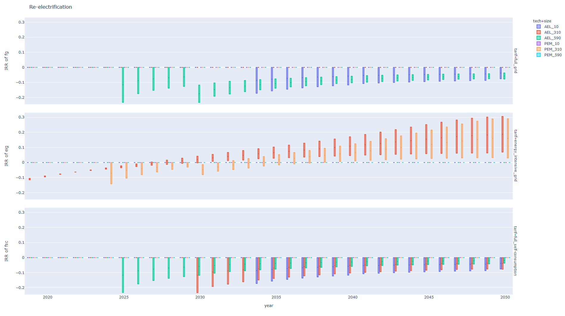
The political determinants are the result of a group Delphi (Hofmaier et al 2018), they are stored in ‘inputs/political_determinants.csv’. The economic determinants base on the irr (internal rate of return) of investments. It is the rate \(\bar{r}_{i,s}\) sucht that for a start year \(i\), an investition \(I_{i,s}\) in sector \(s\) in year \(i\) and a resulting cash flow \(C_{i,s,j}\) over \(25\) years it holds

\[0 = -I_{i,s} + \sum_{j=0}^{25} \frac{C_{i,s,j}}{(1 + \bar{r}_{i,s})^j}.\]

This is computed for all years from 2019 untill 2050 and for all sectors, sizes and technologies. The economic determinant is bounded from above by 1 and bounden from below by 0. It is given by

\[d_{i,s,econ} = \min \left(\max \left(\frac{\bar{r}_{i,s} - l}{u - l},0 \right),1 \right)\]

where \(l\) is the lower bound and \(u\) the upper bound for the return requests of the investor. The economic and political determinats are combined to one determinant \(d_{i,s}\) as weighted sum, in the repository the weights are chosen as 0.6 for the economic determinant and 0.4 for the political determinant. It is assumed that it has 0.06 as lower bound. The combined determinant then is given by

\[d_{i,s} = \min(0.6~d_{i,s,econ} + 0.4~d_{i,s,pol}, 0.06).\]

3. Calculation of the modified diffusion

The modified annual diffusion rate is obatined by damping the annual histroic rate by the determinant,

\[\tilde{r}_{i,s} = d_{i,s} r_{i,s,hist}.\]

With equation (1) the modified capacities can be recursively computed. Note that until 2020 the capacity from the calculaiton of step 1 is used. The capacity is obtained by

\[\tilde{c}_{i,s} = \tilde{c}_{i-1,s} + \tilde{r}_{i,s} \frac{\tilde{c}_{i-1,s}}{1 - \tilde{c}_{i-1,s}}.\]

4. Plotting

At the end the capacities per sector are plotted and compared to the capacities which are calculated from the historic development.

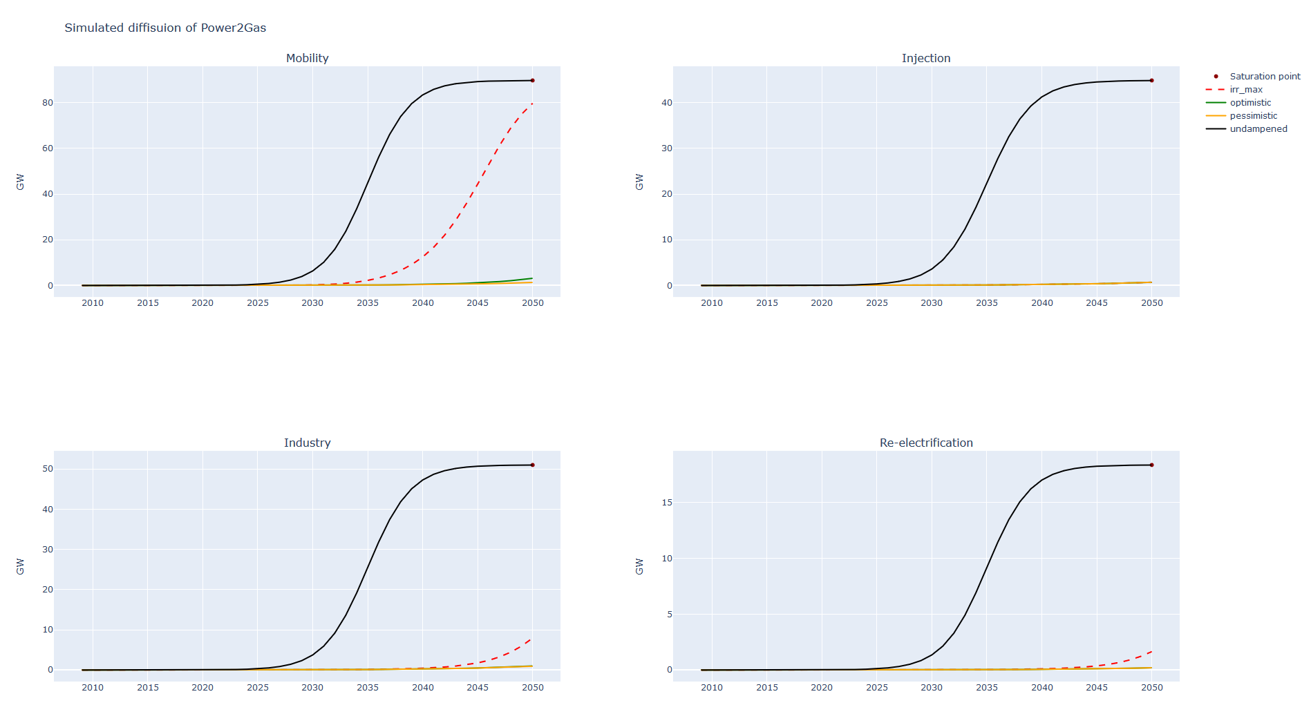
The irr is plotted as well for each technology and facility size.